1. Polynomials drawing pictures
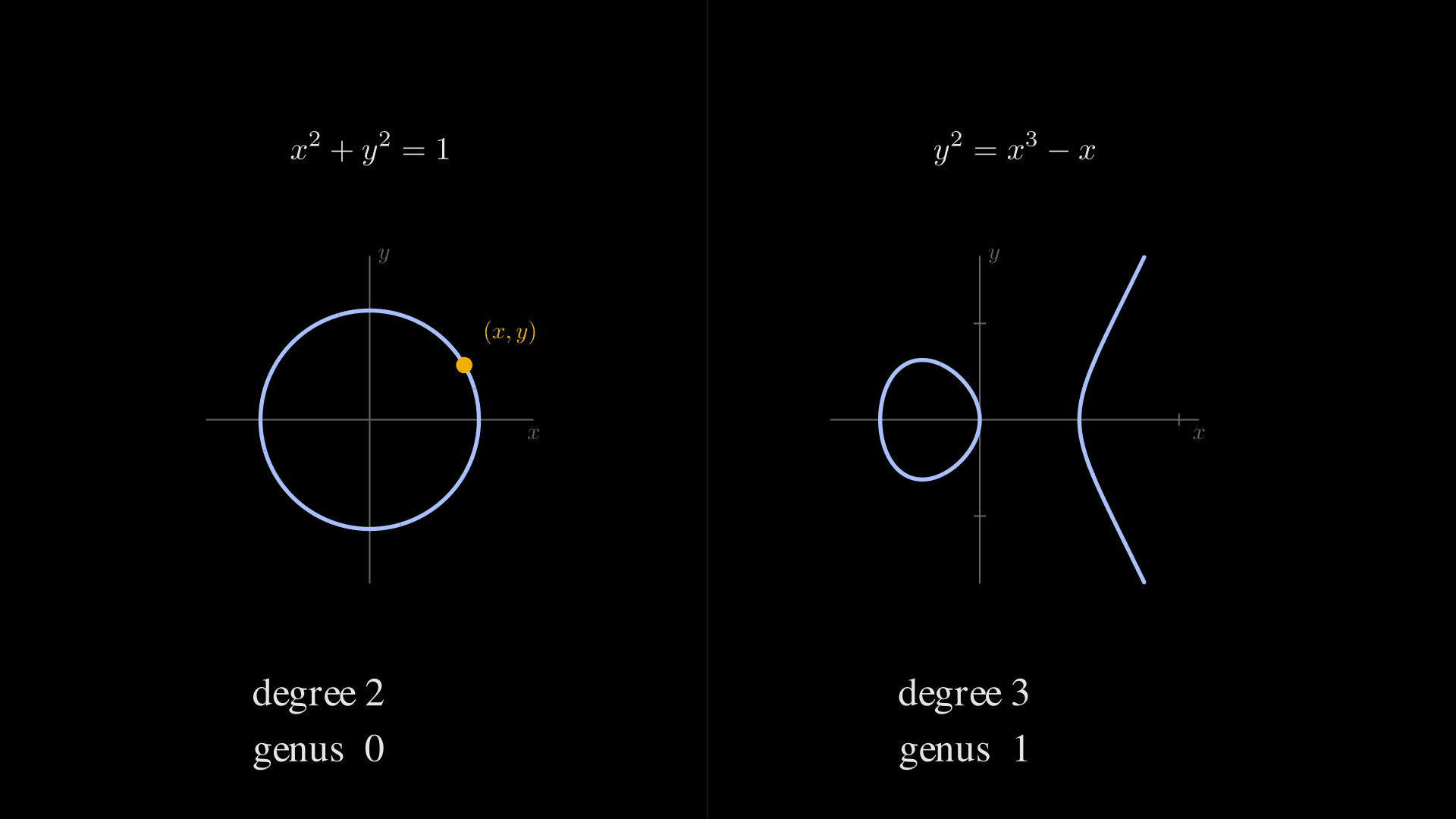
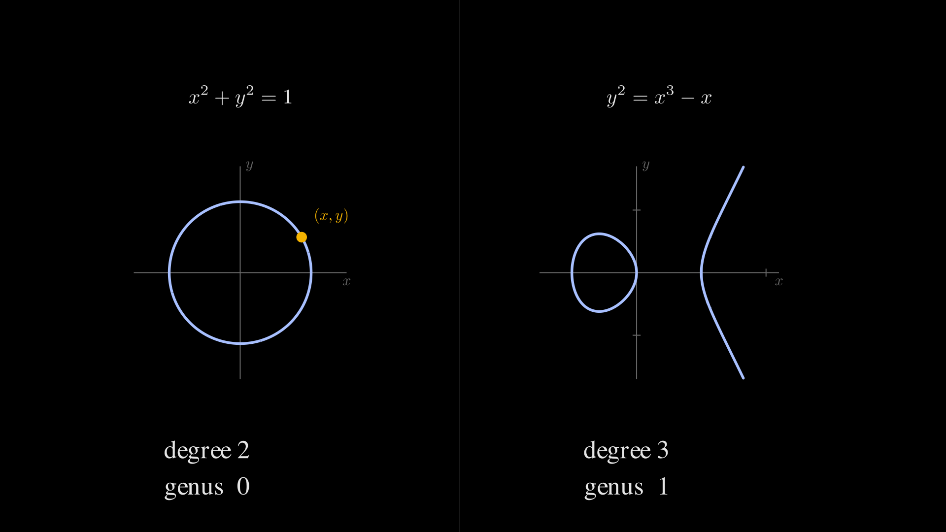
Algebraic geometry studies geometric shapes that arise as solution sets of polynomial equations. The simplest example is the most familiar:
The set of pairs satisfying this equation is a circle of radius one. We have written down a polynomial; it has carved out a curve. That move — from a single algebraic equation to the geometric object it defines — is the seed of the entire subject.
Generalization goes in two directions. More variables and more equations: the equation in three variables defines a sphere, and a pair of equations in three variables generically cuts out a one-dimensional curve, since each equation imposes one constraint and a generic pair imposes two. The second direction is to change the coefficient field. The rest of this article works over the complex numbers, because is algebraically closed — every nonconstant polynomial has as many roots as its degree, and the cohomological machinery we eventually need (Serre duality, derived categories of coherent sheaves, Bridgeland stability) is built on top of that fact. The pictures will continue to be drawn over , but the theorems live over .
A solution set of polynomial equations carved out inside — or, slightly more carefully, inside affine -space — is called an affine algebraic variety. The circle, the sphere, any cubic curve : all are affine varieties, each cut out as the zero locus of a single polynomial in its ambient space. Crucially, an affine variety is not a topological manifold patched from charts. It is a single algebraic object, defined by a single ideal in a polynomial ring, with a single coordinate ring . No gluing is required to define a sphere algebraically; the equation does all the work.
Manim sourceOriginal diagram, rendered with Manim CEOpen full-resolution figure
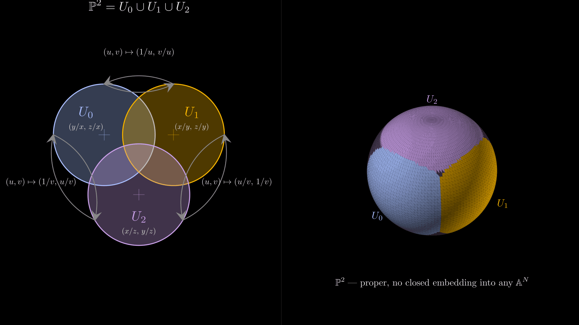
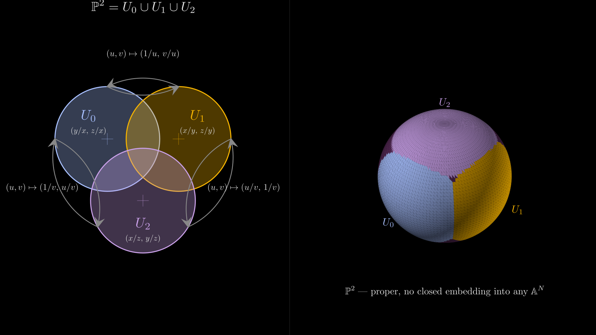
The leap to the modern subject is forced by varieties that genuinely cannot be presented as a single affine piece. The canonical example is projective space : the space of one-dimensional linear subspaces of , parametrizing all "directions" through the origin. Projective space is proper — the algebraic-geometry analogue of compactness — and a basic theorem says that every global regular function on a connected proper variety is a constant. A closed subvariety of an affine space inherits the coordinate functions as global regular functions, and these are not all constant unless the subvariety is a single point. So for cannot be a closed subvariety of any : it has too few regular functions to fit. To work with it, you must build it from pieces — is glued from copies of affine -space along their overlaps, with explicit transition maps relating the homogeneous coordinates. Elliptic curves are projective varieties for the same reason; their group law and cryptographic structure depend on the point at infinity that affine charts on their own cannot see. Once you have one example that demands gluing, you give up trying to embed every variety in some and accept that varieties are objects built by patching affine pieces along common overlaps. The result is the notion of a scheme — a geometric object locally describable by polynomial coordinates, with global topology determined by the gluing data. A scheme is an instruction for gluing affine schemes; the affine ones are the building blocks, projective space is the reason you ever need to build.
Manim sourceOriginal diagram, rendered with Manim CEOpen full-resolution figure
Text description
Once you have schemes, questions multiply: how do you classify them, when are two equivalent, what objects can live on them. Most of this article concerns objects that live on a particular kind of scheme — a smooth projective surface — and how the structure of such objects can become rich enough to ask categorical questions whose answers tell you something deep about the underlying geometry.
2. Enriques surfaces and a nineteenth-century counterexample
The Italian school — Castelnuovo, Enriques, Severi, and others working in Rome and Bologna in the late nineteenth and early twentieth centuries — set the program of classifying algebraic surfaces. A surface here means a complex algebraic variety of complex dimension two, or equivalently a four-real-dimensional space. The classification problem asked two questions: given two surfaces, can you tell whether one can be transformed into the other by birational maps (rational changes of coordinates invertible on a dense open subset)? And which surfaces are rational, meaning birational to projective space ?
Castelnuovo gave a clean criterion: a smooth projective surface is rational if and only if two cohomological invariants vanish:
AsideA first encounter with cohomology
Throughout this article, expressions like appear as vector-space invariants of a variety and a sheaf on it. The reader who has not seen cohomology before can hold onto a single picture, accurate enough to navigate the rest of the article.
Cohomology is the operation you perform when you have a sequence of vector spaces and linear maps satisfying — every composition of two consecutive maps is the zero map. The -th cohomology is then the quotient of "things killed by the next map" by "things produced by the previous map." This single move — kernel of a square-zero operator modulo its image — is the universal pattern of cohomology, and it is pure linear algebra at heart.
For a variety and a sheaf , the groups apply this construction to a complex built from local sections of over an open cover. is the vector space of global sections — pieces of that exist consistently everywhere on . Higher measure obstructions: counts local-to-global glitches (data defined locally that cannot be glued into one global thing); measures obstructions of obstructions.
The reader who has seen vector calculus already knows a special case. A divergence-free vector field on a punctured plane that is not the gradient of any function — circulating around the puncture — represents a nonzero class in of the punctured plane: closed (killed by the next operator) but not exact (not produced by the previous one). Every flavor of cohomology in this article — sheaf cohomology here, the Ext groups in section 3, derived-category cohomology in section 4, and the BRST -cohomology of physics in section 5 — is a variation on this single theme.
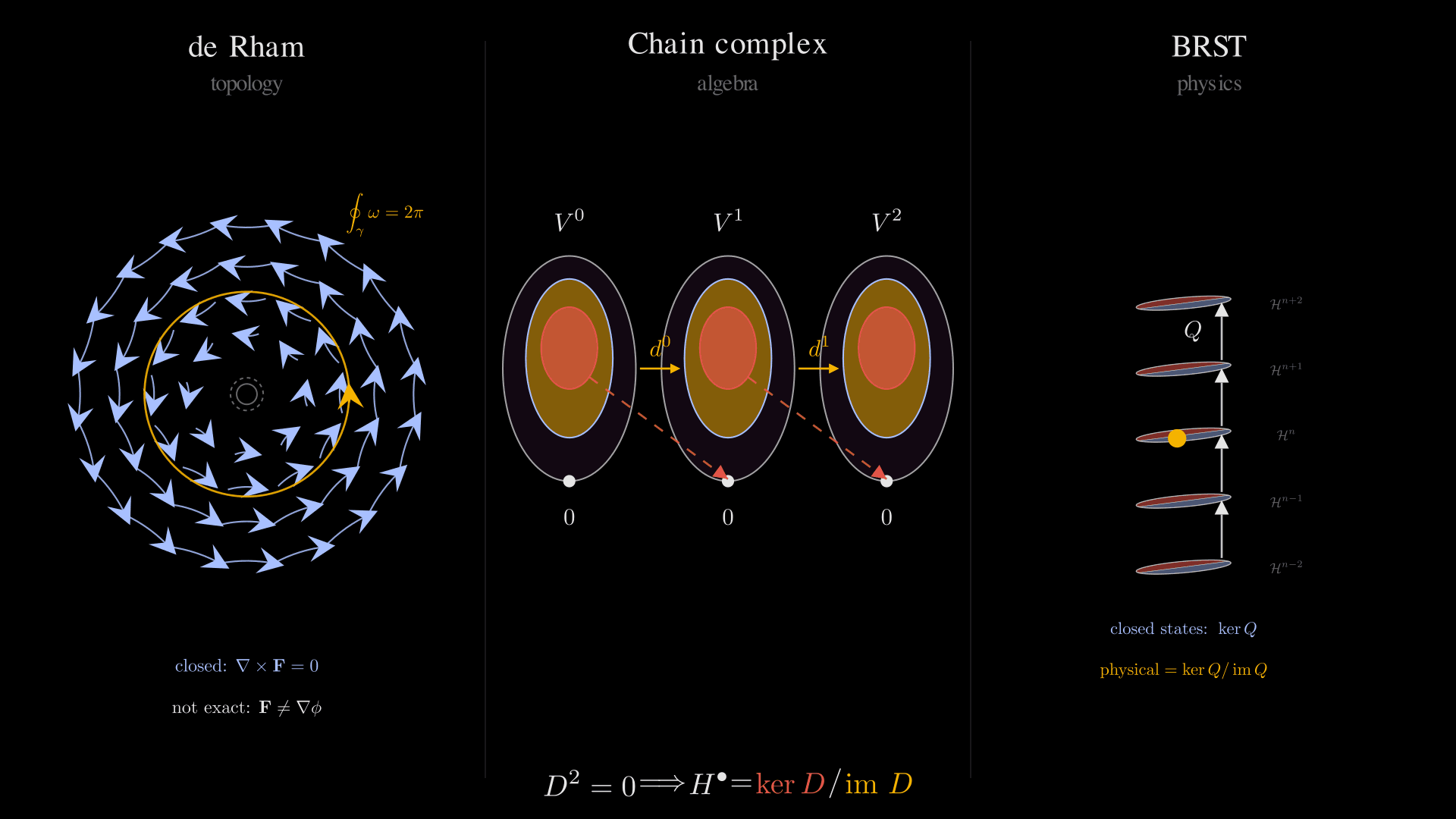
Manim sourceOriginal diagram, rendered with Manim CEOpen full-resolution figure
Text description
Here is the canonical line bundle (the bundle of top-degree differential forms) and is the structure sheaf, both finite-dimensional complex vector spaces once you take their cohomology. Concretely, is the space of holomorphic top-forms on ; measures local-to-global obstructions for holomorphic functions and is harder to describe elementarily, but the Aside above gives the universal picture. The number is the geometric genus; is the irregularity. Castelnuovo's criterion says that vanishing of these two numbers is necessary and sufficient for to be rational, provided you also know the surface is regular — which in this situation turns out to be implied.
Enriques produced a counterexample. He constructed a smooth projective surface — now called an Enriques surface — for which holds but the surface is not rational. His original construction was a sextic surface in passing with multiplicity two through the six edges of the coordinate tetrahedron; the smooth model of that singular surface gave the new example. Vanishing of and does not in itself force rationality — the Enriques surface filled the loophole that Castelnuovo's criterion left open, and it was the first hint that the classification of surfaces was finer than the classification of curves.
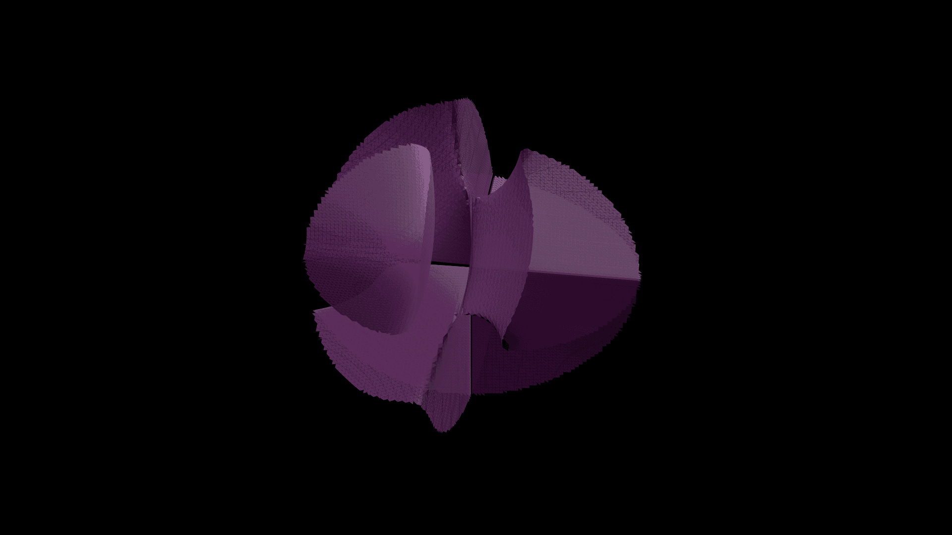
The rendered equation is the Endrass form of the classical sextic at parameter ; the smooth Enriques surface is obtained only after resolving this singular model over .
Manim sourceOriginal diagram, rendered with Manim CEOpen full-resolution figure
The modern definition is cleaner. Over — and more generally over any algebraically closed field of characteristic different from — a smooth projective surface is an Enriques surface if it is minimal (no -curves to blow down), satisfies , and has canonical bundle that is two-torsion:
The non-triviality of is what saves Enriques surfaces from being rational; the two-torsion is what makes them distinctive among all surfaces with vanishing and . Everything in this article runs over , so this is the working definition from here on.
A smooth projective minimal complex surface with and but .
AsideThe characteristic-free definition, and why characteristic 2 is special
The condition with implicitly assumes that the order-two element of corresponding to is carried by the constant group scheme . Over a field of characteristic this is automatic — there is nothing else for it to be. In characteristic , the same order-two class can be carried by an infinitesimal group scheme — or — and when it is, the canonical bundle becomes trivial, , with rather than . These are the singular and supersingular Enriques surfaces; they are bona fide members of the family by every modern test, but our definition above silently excludes them.
The robust formulation, due to Bombieri and Mumford, replaces " two-torsion" with the numerical condition that is numerically trivial, together with and . In characteristic this recovers exactly the definition above; in characteristic it also catches the two extra families. None of the arguments in this article touch characteristic , so the cleaner complex-analytic formulation is what we use.
The two-torsion has a concrete geometric consequence. Whenever a line bundle on a smooth variety squares to the trivial bundle, you can build an unramified double cover of the variety. For an Enriques surface this cover is itself smooth, and it turns out to be a K3 surface — a simply connected surface with trivial canonical bundle and nonzero . An Enriques surface is therefore a K3 surface modulo a fixed-point-free involution; the K3 cover carries strictly more cohomology than the quotient.
where is the deck involution. Enriques surfaces inherit pieces of K3 structure, but only in quotient form, and a great deal of the subject consists of tracking what survives.
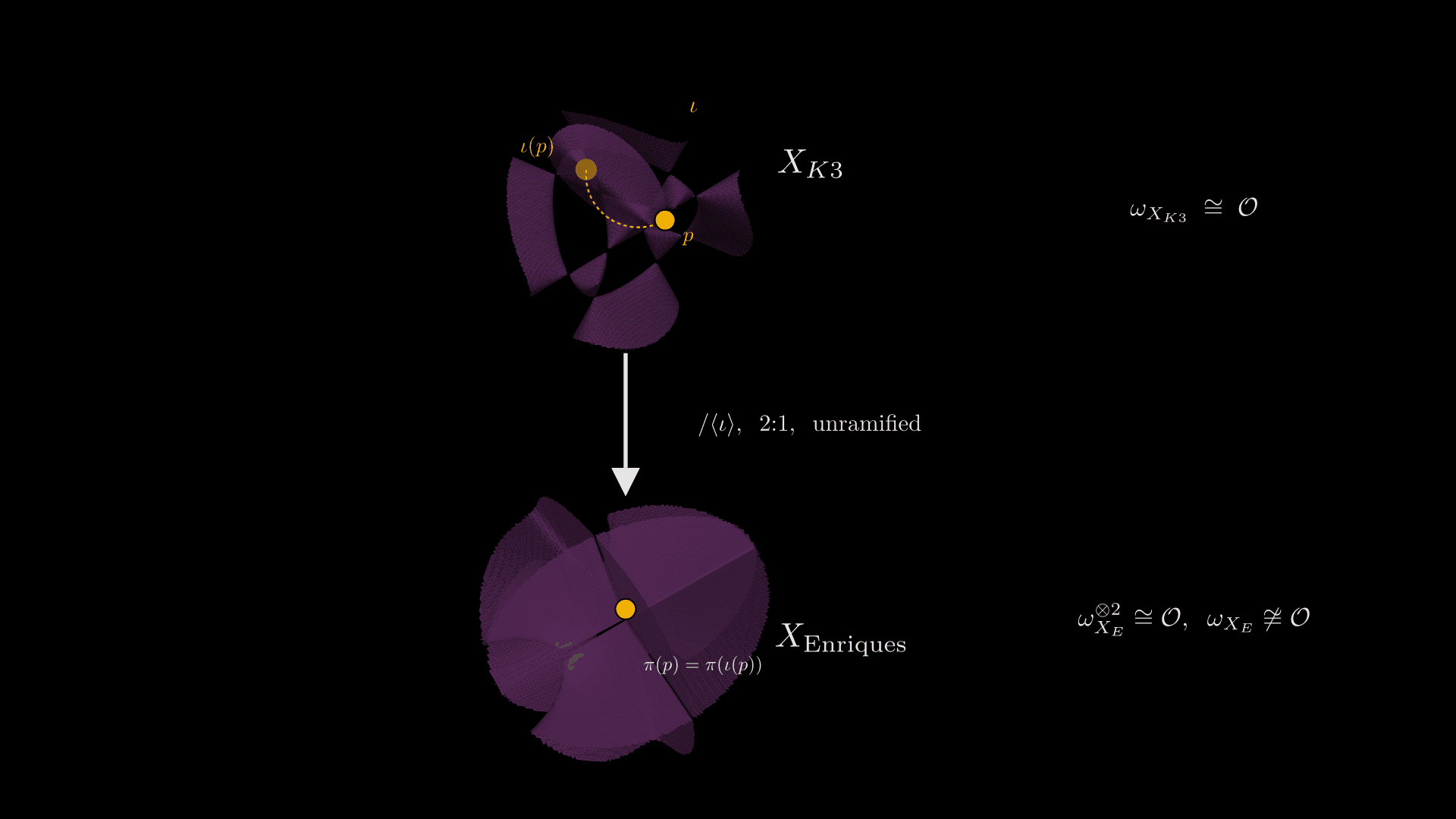
Manim sourceOriginal diagram, rendered with Manim CEOpen full-resolution figure
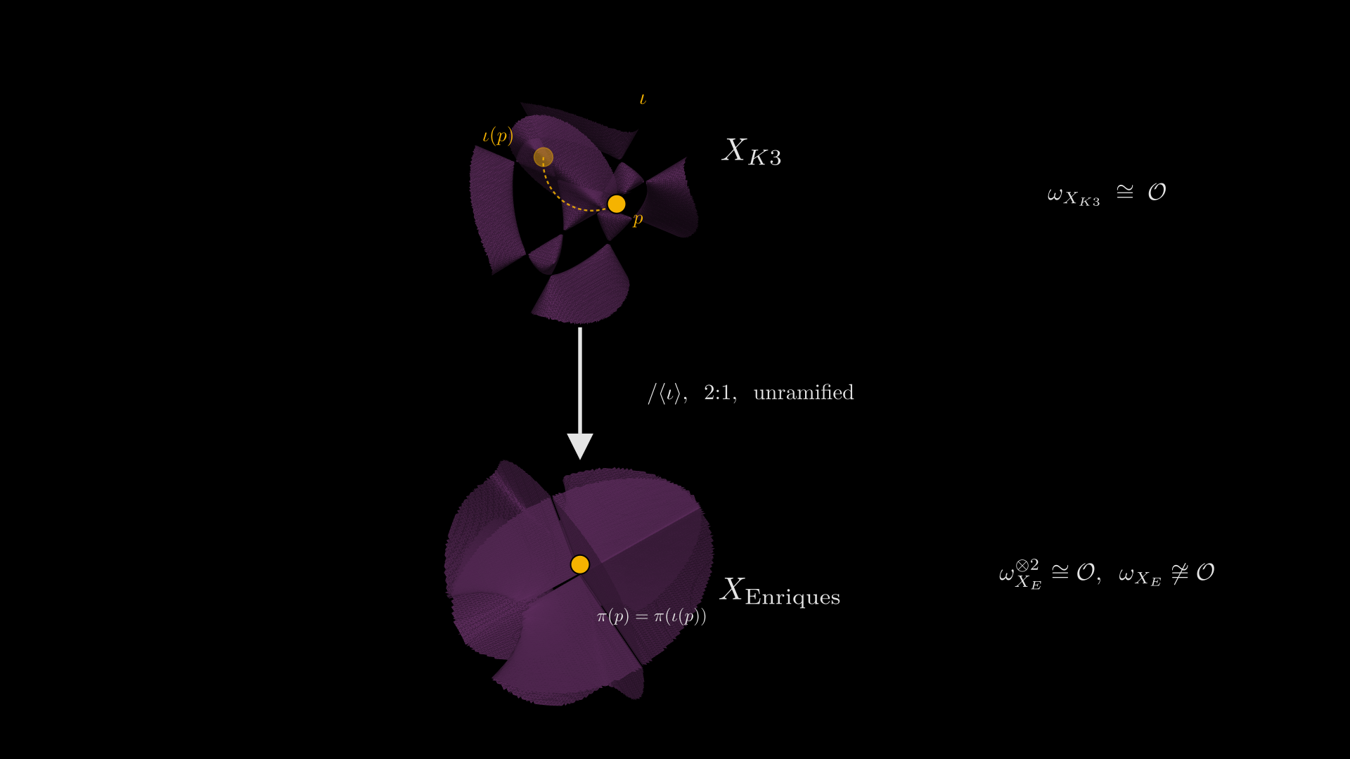
Text description
An Enriques surface can, but need not, contain rational curves. A smooth rational curve on a surface has self-intersection , because it is a smooth embedded with normal bundle ; such curves are called -curves. A generic Enriques surface contains none at all — these are called unnodal or generic, and they are the cleanest representatives of the family.
The unnodal hypothesis buys the cleanest picture: on a generic surface the ten line bundles of section 6 are completely orthogonal, and the Kuznetsov component has its simplest description. It is not what the final theorem depends on. On a nodal surface the same ten line bundles still exist and are still exceptional, but they organize into orthogonal blocks whose members differ by chains of -curves (Li–Stellari–Zhao), and the non-existence argument at the end of this article runs block by block with no change (Corollary 8.5). We work in the unnodal case throughout for clarity, not out of necessity.
3. Vector bundles and coherent sheaves
To do anything with a variety beyond classifying it up to isomorphism, you put stuff on it. The most basic stuff is a vector bundle: a continuous (in our case, holomorphic and algebraic) family of vector spaces parametrized by the points of the variety. The tangent bundle of a smooth variety assigns to each point the tangent space there; the canonical bundle assigns to each point the one-dimensional space of top-degree differential forms. A line bundle is a vector bundle whose fibers are one-dimensional.
The algebraic way to package a vector bundle is as a locally free sheaf: a sheaf on such that on each small open subset , the sections form a free module over the ring of regular functions . "Locally free" expresses the bundle's local triviality; the global structure is captured by how the local trivializations glue.
This is enough for many purposes, but the category of vector bundles has a fundamental defect: it is not abelian. A morphism of vector bundles is a fiberwise linear map, and the kernel and cokernel can fail to be vector bundles — because the rank of the map can jump at certain points. Take a map given by multiplication by a section vanishing along a curve; the cokernel is supported on that curve, where it is one-dimensional, and zero everywhere else. A "vector space that vanishes outside a subvariety" is not a vector bundle.
To fix this we generalize. The right object is a coherent sheaf — and on the schemes we care about, the working description is that a coherent sheaf is, locally, the cokernel of a map between two free -modules of finite rank. This local-cokernel condition is what is technically called finitely presented; it agrees with coherence on a Noetherian scheme, and every variety considered in this article is Noetherian. Coherent sheaves form an abelian category: kernels and cokernels stay coherent, and exact sequences make perfect sense. Vector bundles sit inside the coherent sheaves as the locally free sheaves of finite rank, but they are no longer the only objects.
Let be a Noetherian scheme. A sheaf on is coherent if every point has an open neighborhood such that is the cokernel of a morphism between free sheaves of finite rank. (On non-Noetherian schemes the definition splits from finite presentation; we will not encounter that subtlety.) Coherent sheaves form an abelian category .
A skyscraper sheaf supported at a point assigns the field to any open set containing and zero to any open set not containing . It is coherent — locally it is the cokernel of the inclusion of the maximal ideal — but not locally free, because its rank jumps from one to zero as you move off the point. An ideal sheaf of a subvariety consists of regular functions vanishing along ; it is the kernel of the surjection , and it is coherent and torsion-free, but not locally free unless is a divisor (a codimension-one subvariety—like a curve on a surface—that is locally defined by a single function).
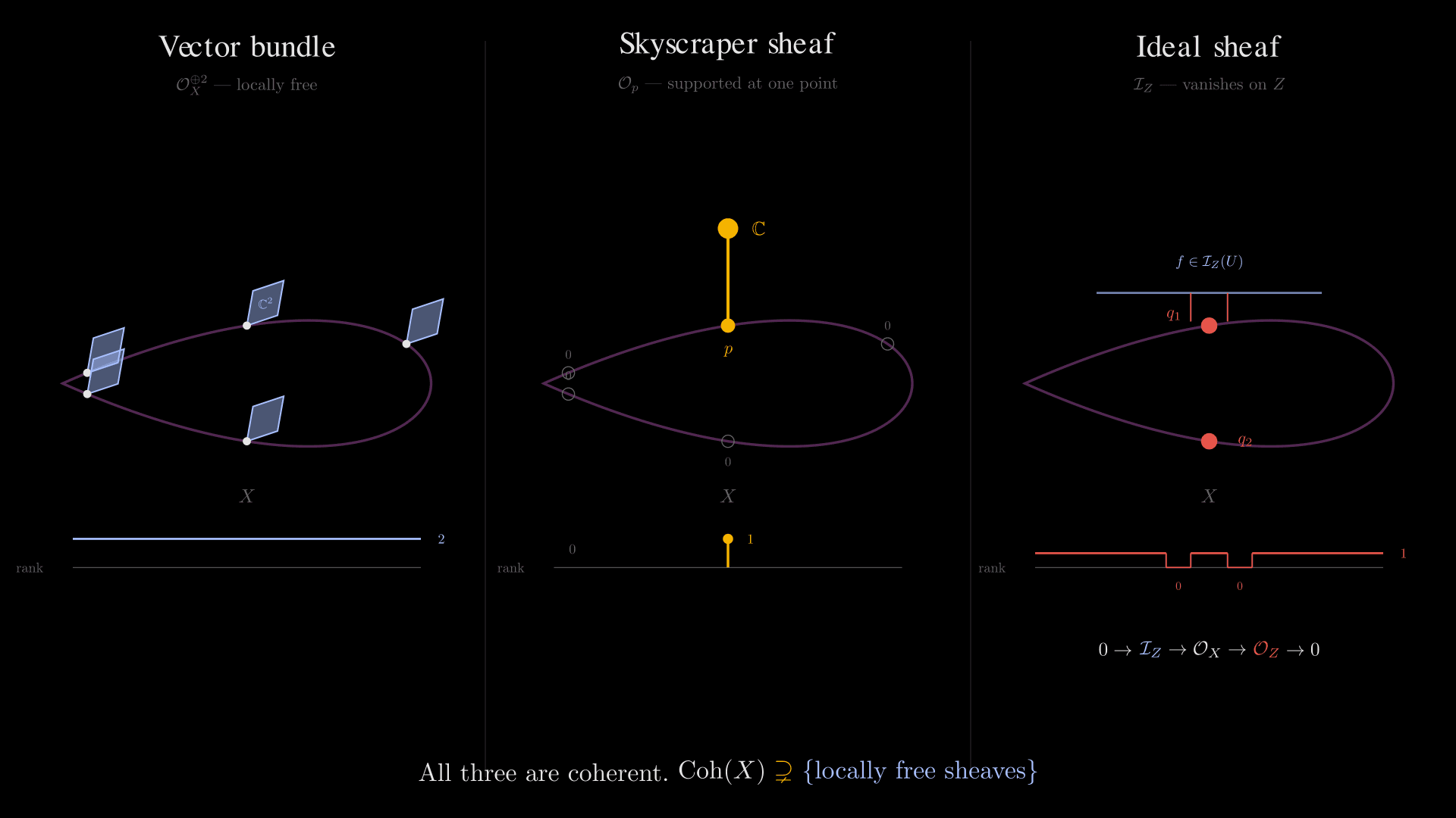
Manim sourceOriginal diagram, rendered with Manim CEOpen full-resolution figure
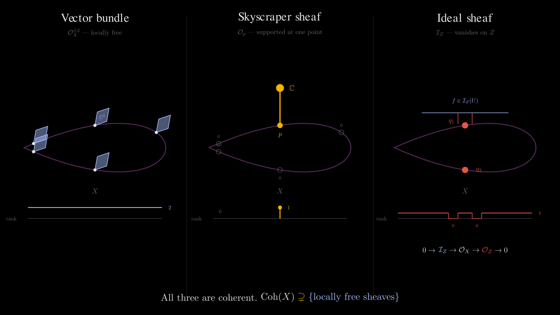
Text description
These are exactly the sheaves that physicists call -branes (skyscrapers) and -branes wrapping cycles (ideal sheaves), as we will see in section 5. The fact that contains them all on equal footing is what makes it the right setting for both algebraic geometry and string-theoretic D-brane computations.
4. Complexes and the derived category
Coherent sheaves are abelian, but still not enough. For deeper invariants — cohomology, derived functors, the homological invariants that appear in moduli problems — you need to consider not just individual sheaves but complexes of sheaves.
A complex of coherent sheaves is a sequence
where the morphisms compose to zero, . This is the same square-zero condition we just met in the cohomology Aside of section 2, now applied to bundle-like objects rather than abstract vector spaces; the differential is a morphism of sheaves, but the formula behind every flavor of cohomology in this article is the same. The cohomology of the complex at degree is , again a coherent sheaf. A complex is bounded if only finitely many of the are nonzero. The whole machinery of homological algebra rests on the recognition that the complex carries more information than its cohomology, but the appropriate equivalence relation makes complexes indistinguishable when they have the same cohomology.
That equivalence relation is quasi-isomorphism: a morphism of complexes inducing an isomorphism on every cohomology group. The bounded derived category of coherent sheaves, , is the category of bounded complexes with quasi-isomorphisms formally inverted. An object of is a bounded complex; a morphism is a "roof" where the left arrow is a quasi-isomorphism. Coherent sheaves embed into as complexes concentrated in a single degree.
The derived category has two structural features distinguishing it from an abelian category. First, the shift functor translates a complex one position to the left:
It is invertible, with inverse , and applying repeatedly gives an action of on . Second, short exact sequences of complexes get replaced by distinguished triangles:
A distinguished triangle is the derived-category analogue of a short exact sequence. Long exact sequences in cohomology come out of distinguished triangles, and most structure theorems of algebraic geometry translate naturally into this language. The derived category equipped with its shift and its distinguished triangles is the prototypical example of a triangulated category, the abstract setting for the rest of this article.
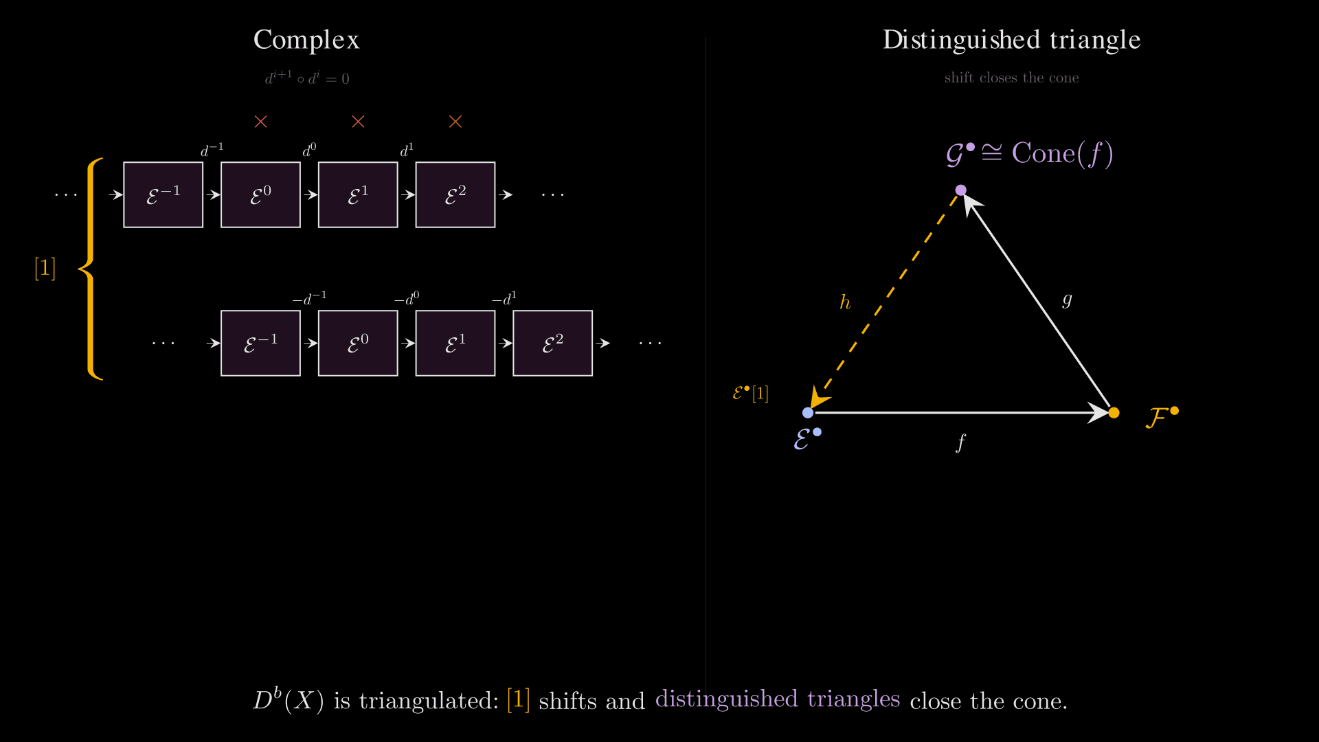
Manim sourceOriginal diagram, rendered with Manim CEOpen full-resolution figure
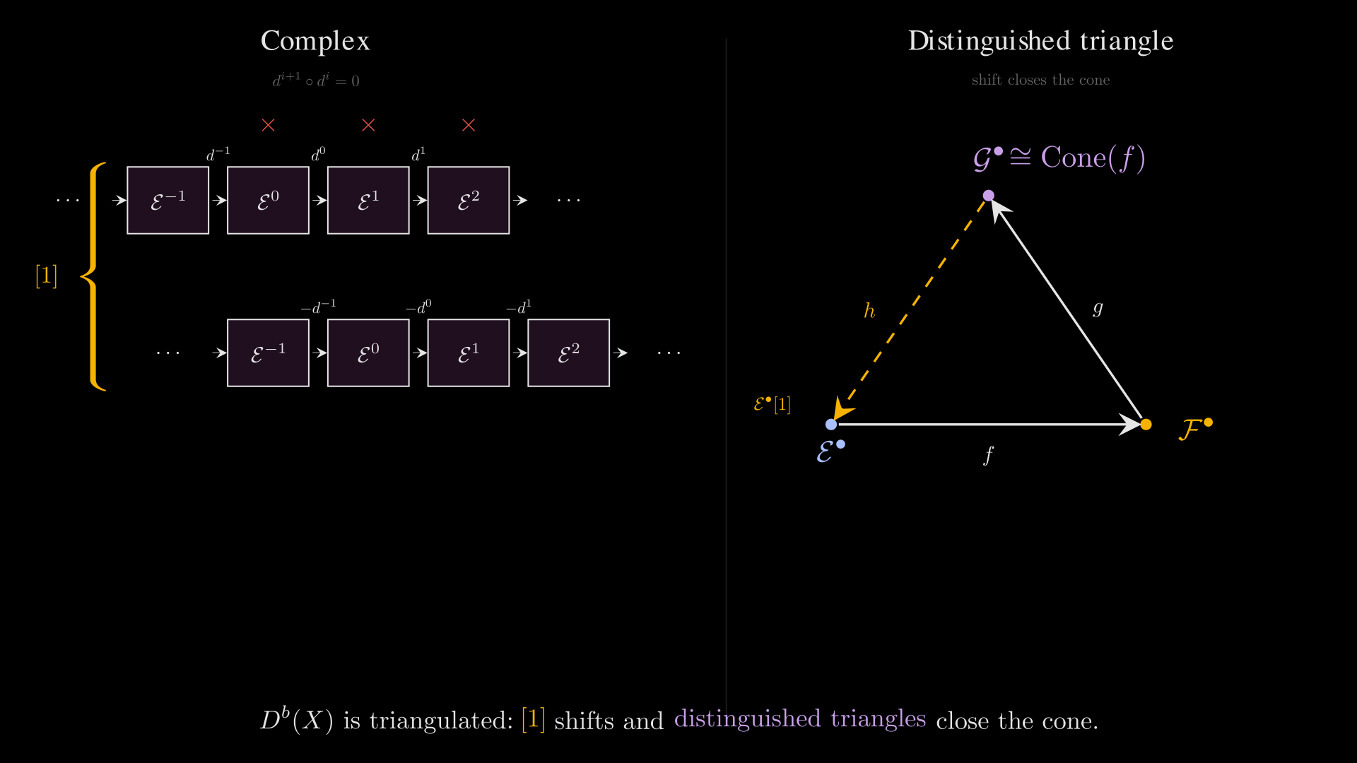
Text description
Let be a smooth projective variety of dimension over . There is a functor , the Serre functor, given by satisfying a natural perfect pairing . Equivalently, in form: for ,
The Serre functor is the categorical incarnation of Serre duality — and it is the operator whose interaction with stability conditions will produce our final contradiction. For an Enriques surface, and is two-torsion, so
The Serre functor squares to the homological shift by four. On a K3 surface the Serre functor is just (because ), so it commutes with everything; on an Enriques surface it carries genuine torsion information — which is why the Enriques case is rigid in a way the K3 case is not.
Two bookkeeping consequences for — the abstract Grothendieck group whose elements are formal -linear combinations of coherent sheaves modulo short exact sequences — will be used repeatedly. First, a distinguished triangle gives the additivity relation in . Second, the class of a bounded complex equals the alternating sum of the classes of its cohomology sheaves:
This recipe is what converts the cohomology-sheaf description of a complex into a numerical class; together with additivity on triangles, it is how every class in sections 6 and 8 is computed.
Why does any of this matter? The mathematician's answer is the homological algebra of varieties. The physicist's answer is more striking — and it is what convinced algebraic geometers they were studying the right object.
5. B-branes, the topological string, and Q-cohomology
There is a question that mathematicians of the 1990s could not have answered cleanly without help from physics: why is the derived category of coherent sheaves the right invariant of an algebraic variety, rather than just the abelian category of coherent sheaves? Coherent sheaves are abelian, geometrically natural, and sufficient for many purposes. What forces us to enlarge them to a triangulated category?
The answer came from a class of two-dimensional quantum field theories called topological string theories. The story begins with the type II superstring on a Calabi-Yau target, but you can read what follows as a structural argument that any reasonable notion of "what lives on " forces you to the derived category — even without committing to string theory.
Aside$Q$-cohomology: cohomology in physics
Before diving into topological strings, a physical analogy worth pinning to the cohomology Aside in section 2.
In quantum field theories with a fermionic gauge symmetry, one frequently has a square-zero operator acting on the Hilbert space of states: . Physical states are taken to be elements of — states "-closed" in the sense of being annihilated by — modulo elements of , which are deemed gauge-equivalent to zero. The space of physical states is therefore This is exactly the cohomology construction we have been using. The operator plays the role of the differential ; the condition is the same as ; "physical states modulo gauge" is "kernel modulo image."
The classic prototype is electromagnetism. The gauge transformation is the image of an exterior derivative, the physical field strengths are the closed forms, and the gauge group of -fields modulo gradients is, on a topologically nontrivial spacetime, exactly the de Rham cohomology of that spacetime. The BRST formalism systematizes this: any time you have a gauge symmetry, you can construct a such that and physical states are -cohomology classes.
In the topological string below, is one of the worldsheet supercharges, promoted to a scalar by the topological twist. Open-string states between two D-branes will turn out to be -cohomology groups, and we will see that mathematically these are the Ext groups — yet another flavor of the same kernel-mod-image construction, now applied to coherent sheaves. The thread "cohomology equals kernel mod image of a square-zero operator" runs through every formal object in this article.
A Calabi-Yau threefold supports a sigma model with supersymmetry on the worldsheet. Witten's topological twist of this theory comes in two flavors, the A-twist and the B-twist, distinguished by which combination of worldsheet supercharges you promote to a worldsheet scalar. The B-twist is consistent precisely when , the Calabi-Yau condition. After twisting, one supercharge becomes a worldsheet scalar nilpotent operator , the BRST operator, satisfying
Physical observables are -cohomology classes — equivalence classes of states satisfying ("-closed") modulo states of the form ("-exact"). This is the same kernel-mod-image computation as in section 4; the BRST operator is the , and physical states are the cohomology in the linear-algebra sense above. Correlation functions in the B-model depend only on the complex structure of and not on its Kähler structure. The closed-string state space is the Dolbeault cohomology , packaged more invariantly as the Hochschild cohomology of .
The question sharpens when you allow worldsheets with boundary — which physicists must, because that is what describes open strings ending on extended objects called D-branes.
A worldsheet with boundary needs boundary conditions to make the variational problem well-posed. Witten's analysis of B-model boundary conditions shows that they amount to a choice of complex submanifold of together with a holomorphic vector bundle on it. The conclusion: a B-brane is a holomorphic vector bundle on , and the open-string spectrum between two B-branes and is
The right-hand side is a finite-dimensional complex vector space — the Ext groups of and . For , is just the linear bundle maps from to ; for higher , measures "-step extensions" of by and is itself an instance of the kernel-mod-image construction we have been tracking. The cohomology groups from section 2 are the special case — Ext is a generalization of cohomology, with the structure sheaf in the first slot replaced by an arbitrary sheaf. The open-string ghost number matches the homological degree, and the worldsheet -cohomology of operators between branes lands exactly on this .
That would be satisfying if it were complete, but three physical phenomena push the formalism further. Singular branes: a D-brane wrapped on a point (a "-brane") is a skyscraper sheaf, not a bundle, and a brane consisting of an ideal sheaf of a subvariety is a coherent sheaf that is not locally free. Anti-branes: a brane and its anti-brane have opposite orientations, so you need formal additive inverses. Tachyon condensation: a brane and antibrane with an open-string tachyon can decay to a bound state, and Sen's tachyon condensation analysis identifies that bound state with the mapping cone — a complex of branes, not a single brane. Multi-step bound states give complexes of arbitrary length.
Coherent sheaves handle the first phenomenon. Triangulated structure — shifts, cones, quasi-isomorphism as gauge equivalence — handles the second and third. The natural closure of "holomorphic bundle" under these physical operations is exactly .
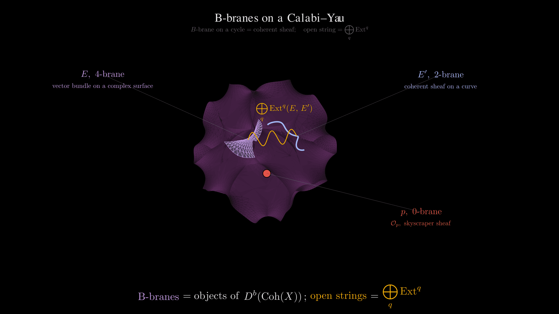
Manim sourceOriginal diagram, rendered with Manim CEOpen full-resolution figure
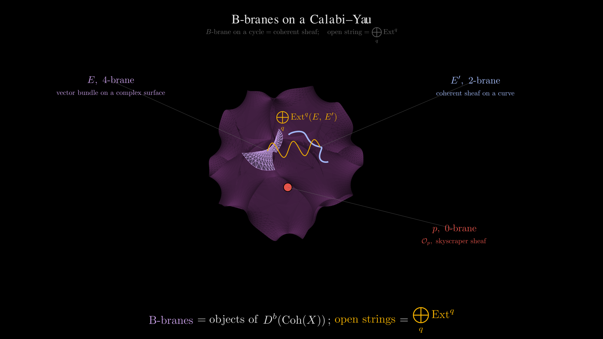
Text description
Douglas's 2001 proposal is that the category of B-type D-branes on a Calabi-Yau is the bounded derived category of coherent sheaves. This sits inside Kontsevich's 1994 Homological Mirror Symmetry conjecture, which predicts an equivalence
between the B-side category on and the Fukaya category on the mirror , trading complex geometry for symplectic geometry. For mathematicians, the conjecture was the first strong hint that the derived category was the structurally correct object on the algebraic side.
The key dictionary entry for our purposes:
Once you accept that the right object is , you can ask physical questions about which branes are stable — which actually exist as BPS states at a given point of moduli space. Douglas formalized this as -stability, with branes carrying a phase determined by the period of the holomorphic three-form. Bridgeland, in 2007, gave a clean mathematical version: a stability condition on any triangulated category. The Enriques surfaces we care about are not Calabi-Yau, but the formalism extends, and what started as a physics motivation for becomes an algebraic-geometric tool for studying Kuznetsov components.
6. Exceptional collections and the Kuznetsov component
Let be a generic (unnodal) complex Enriques surface with derived category . The goal here is to carve into pieces, isolating the component on which the final argument will run.
The cleanest pieces of any derived category are those generated by exceptional objects.
An object is exceptional if and for every . Equivalently, has only scalar endomorphisms and no self-extensions in any nonzero degree.
A short calculation shows that on an Enriques surface, every line bundle is exceptional. Given a line bundle , the self-Ext groups are
The first equality uses that on a smooth variety equals the cohomology of the bundle , which is the trivial bundle . The second equality just rewrites the trivial bundle as . The right-hand side is now exactly the cohomology Castelnuovo's criterion was about: for (global constants on a connected variety), zero for (since ), and zero for (since ). Every line bundle is exceptional.
What is special to the unnodal case is that one can find a particularly clean exceptional collection.
For a generic (unnodal) Enriques surface, there is a collection of ten line bundles on that is completely orthogonal: for every pair and every integer ,
The construction is lattice-theoretic. The Picard lattice of a generic Enriques surface is the rank- Enriques lattice , and one finds ten isotropic divisor classes with intersection numbers ; the line bundles built from these classes give the orthogonal collection. The vanishings for rest on Riemann–Roch and vanishing arguments that fail in the presence of -curves — this is exactly where the unnodal hypothesis enters.
The next piece of categorical scaffolding is the semiorthogonal decomposition.
A semiorthogonal decomposition is a sequence of full triangulated subcategories such that for , and is generated by the as a triangulated category.
With ten orthogonal exceptional line bundles, we get
where is everything left over.
The Kuznetsov component of a generic Enriques surface is the right orthogonal complement
Concretely, consists of complexes whose hypercohomology against every vanishes in every degree — the part of that does not see any of the ten chosen line bundles.
AsideThe numerical Grothendieck group $K_{\mathrm{num}}$
For a triangulated category , the numerical Grothendieck group is the quotient of the abstract Grothendieck group by the kernel of the Euler pairing The quotient is always torsion-free: the map embeds it in . For it has rank . The semiorthogonal decomposition splits the rank- lattice as the direct sum of the rank- sublattice spanned by and its orthogonal complement — orthogonal in both directions, because the Euler form of an Enriques surface is symmetric (Lemma 7.4). Under the Mukai pairing the ambient lattice has signature , and the ten classes span a negative-definite sublattice (), so is positive definite on the rank- complement: a class with is zero. Lemma 6.8 uses this definiteness once, as a cross-check, and does not use torsion-freeness at all.
The rank of is therefore , sitting as the orthogonal complement of the rank- sublattice spanned by inside the rank- ambient lattice.
Code-native SVG sourceOriginal diagram, rendered by the shared article system
Text description
Because each is admissible, the inclusion has both a left adjoint and a right adjoint . Both are projections onto and both restrict to the identity there, but their values on ambient objects can differ. The triangles below identify which projection is being used. Erratum 9.1 records the correction to the adjoint conventions.
The left adjoint is the left mutation through the collection. For there is a distinguished triangle
whose first arrow is evaluation. The cone lies in : applying to the triangle, complete orthogonality makes the first arrow an isomorphism, so the third term is killed. It is the left adjoint because applying for kills the first term (as ) and leaves . In the standard notation for mutations, .
The right adjoint is also a mutation, but through the twisted collection. Serre duality on gives , so the same subcategory has two descriptions,
and the projection onto the left orthogonal of is the right mutation
Applying for kills the third term and gives , the right-adjoint property. In mutation notation, , the right mutation through the twisted collection regarded as an endofunctor of .
We will frequently abbreviate as when the indexing is clear from context.
The two adjoints differ on exactly the objects that matter below. The left adjoint kills the collection, , while is the 3-spherical object of Theorem 6.7. The right adjoint kills the twisted collection, (because by the Serre duality above), while is a shift of that same spherical object.
Let be an admissible subcategory of a triangulated category with Serre functor . Then has a Serre functor, given by
The proof is one line: for , . The formula for the inverse is the same computation with the other adjoint. Bondal–Kapranov's 1989 paper on Representable functors, Serre functors, and mutations is the source; Li–Stellari–Zhao (arXiv:2104.13610, Remark 1.1) state exactly this form.
For the Enriques component, with and ,
The two formulas look alike and are easy to confuse: the evaluation-cone functor computes the inverse Serre functor up to the shift , not the Serre functor. On the spherical objects below the difference is a shift by two — the Serre functor gives , the evaluation-cone functor gives .
Squaring in the ambient kills the torsion in , giving ; in the terminology of Li–Nuer–Stellari–Zhao, is a -Enriques category. The component is not. Writing and conjugating the inner mutation by ,
a shift only up to a mutation autoequivalence, and on the spherical objects below acts as , not . The Serre functor of is not a shift: a shift would have to be by Theorem 6.7, and Lemma 8.1 below would then force for every class in the rank-two lattice . Whether is a shift is a different question, which the argument below does not need. That is the algebraic remnant of the two-torsion of , and it is what generates the obstruction in section 8.
One more object is needed. There is a recipe that produces 3-spherical objects in from the line bundles of the collection. The notion of an -spherical object is due to Seidel and Thomas, and it requires two conditions — a Calabi-Yau- condition on the Serre functor, and a constraint on the endomorphism algebra that identifies it (as a graded vector space) with the singular cohomology of the -sphere.
Let be a -linear triangulated category with Serre functor , and fix an integer . An object is -spherical if it satisfies both:
-
Endomorphism algebra. The graded -algebra of is isomorphic, as a graded -vector space, to the singular cohomology of the -sphere: Concretely, , , and for .
-
Calabi-Yau- condition. .
The case — a 3-spherical object — is the one relevant to .
For each , Serre duality gives , so there is a unique nonzero morphism up to scalar. Let be its cocone: Then:
- , and .
- is a nonzero 3-spherical object of : and .
- The are pairwise orthogonal: for .
The parts that the rest of the article uses are short enough to prove here.
lies in . Apply to the defining triangle. For , both and vanish, by complete orthogonality and Serre duality — this is the "twisted vanishing" for , and it needs no separate lemma. For , any nonzero map induces an isomorphism , because both sides are one-dimensional and concentrated in degree . Either way .
. In the right-mutation triangle for , the coefficient is for and zero otherwise, so the triangle reads . Its second arrow is nonzero — were it zero, would contain as a direct summand and could not lie in — and since , every nonzero arrow has the same cocone up to isomorphism: the defining triangle of .
. Apply to the defining triangle to get , then apply . The middle term dies, , because ; the last term becomes . So .
The computation and the orthogonality are Lemma 4.8 of arXiv:1912.04332; the identification is their Remark 4.9(ii), and is their equation (4.2) (they write for our ). See Erratum 9.4 for the bibliographic corrections.
For each , in .
The defining triangle gives in , and in because in rational cohomology (the Aside below). So in , of which is a direct summand. As a cross-check, , and the Euler form is definite on the rank-two lattice , so an isotropic class must vanish.
This lemma is the pivot of section 8. A nonzero semistable object always has nonzero central charge, so a numerically trivial object can never be semistable: under any numerical stability condition on , Serre-invariant or not, each is unstable and has a Harder–Narasimhan filtration with at least two pieces.
AsideThe algebraic Mukai lattice and $\mathrm{ch}(\omega_X) = 1$
The Mukai vector is the Chern character multiplied by the square root of the Todd class:
Here , , and . Degree-four classes are written as their degree, with the point class as generator. Inside , the image of this map is the algebraic Mukai lattice:
The last coordinate is tied to the rank: is integral when is even and half-integral when is odd. Indeed, the Enriques divisor lattice is even, so has integral degree; additivity extends this statement from bundles to complexes. For example, and , whereas is not an allowed class. See Nuer, arXiv:1406.0908, section 3, for the Mukai-vector convention; Erratum 9.3 explains the necessary parity constraint in the integral lattice.
In these coordinates the Mukai pairing is
It is integral on the displayed lattice: writing and makes an integer. The variable is a Mukai coordinate; the Riemann–Roch computation in Lemma 7.4 instead uses , so .
Because is two-torsion, in rational cohomology, and Thus , and tensoring by acts as the identity on . This equality of numerical classes does not identify the objects and . In particular, it does not identify the ambient Serre functor with the intrinsic Serre functor of the Kuznetsov component.
7. Bridgeland stability conditions
The reason this notion exists in the first place is physics. Section 5 explained why D-branes on a Calabi–Yau live in ; the next question, the one that drove the subject in the late 1990s, was: which of those objects actually exist as physical states? Not all of them. A D-brane wrapping a cycle has a mass; for the brane to be a stable particle in the four-dimensional effective theory, that mass has to be locked in place by the supersymmetry algebra, not just by dynamics. The objects for which this happens are the BPS states, and the algebra of stability conditions is the language that catches them.
In type II string theory compactified on a Calabi–Yau threefold, the resulting four-dimensional theory has supersymmetry — eight supercharges, with a complex central charge extending the algebra and depending on the charge of the state. On the IIB side is the period of the holomorphic three-form over a 3-cycle; on the IIA side is built from the complexified Kähler class together with the brane charge. Either way, a representation-theoretic calculation gives the BPS bound
with equality on short multiplets. The states that saturate this bound — annihilated by half of the supercharges — are the BPS states. They cannot decay into lighter states of the same total charge because the bound forbids it; their stability is built into the algebra rather than the dynamics.
Bound states obey a triangle inequality. If a BPS state of charge is composed of constituents of charges , the central charge is additive but the mass is sub-additive:
with equality precisely when the two phases align. The deficit between the two sides is the binding energy. As the moduli of vary — Kähler class on the IIA side, complex structure on IIB — the central charges rotate in , and across real-codimension-one walls of marginal stability their phases align. On one side of the wall the bound state is BPS; on the other it has decayed into its constituents. The natural angular variable to track is the BPS phase , and the discontinuous reorganization of the spectrum across walls is the phenomenon called wall-crossing.
Michael Douglas, in a sequence of papers culminating in his ICM 2002 lecture, translated this picture into the language of triangulated categories. A distinguished triangle in describes as a tachyon condensation bound state of and . The state is -stable (the stands for period) when, for every such triangle with nonzero, the BPS phases satisfy
This single inequality re-encodes the mass-deficit picture entirely: a sub-brane of smaller phase contributes mass that locks into the sum constructively, leaving binding energy on the table; if the phases ever cross, the bond breaks. -stability varies continuously across the Kähler moduli space, the spectrum jumps at walls, and the worldvolume gauge theory on undergoes a corresponding change of quiver and superpotential.
Bridgeland's 2007 axiomatization is the rigorous mathematical version. The dictionary is exact: the heart of a bounded t-structure is the categorical incarnation of "which objects count as particles versus antiparticles" at a given point of moduli space; the central charge is a linear function on the Grothendieck group, realized for Calabi–Yau examples by the same period integrals that appear in the physics; the phase is the BPS phase; the Harder–Narasimhan filtration is the unique decomposition of any object into elementary semistable factors of strictly decreasing phase, mathematically formalizing the existence of a well-defined BPS spectrum; and the support property is what makes the moduli space of stability conditions — denoted — a complex manifold rather than a wild set, so that one can deform continuously in the way the physical Kähler moduli demand. Conjecturally, a connected component of the space is the universal cover of the stringy Kähler moduli space of — the moduli that string theory says is the true parameter space for the B-model. Donaldson–Thomas invariants count -semistable objects and recover BPS state counts; the Kontsevich–Soibelman wall-crossing formula matches the physical spectrum jumps to the categorical operations of tilting a heart at a torsion pair.
With the physical picture as backdrop, we now state the axioms for a triangulated category — applied throughout to , but everything generalizes.
A stability condition on is the data of:
- The heart of a bounded t-structure (an abelian subcategory).
- A central charge , a group homomorphism on the Grothendieck group, satisfying:
- Positivity. For every nonzero , .
- Existence of Harder–Narasimhan Filtrations. Every nonzero admits a unique filtration with semistable factors of strictly decreasing phases .
For nonzero , the phase is
The phase is the angular position of in the upper half-plane, normalized so that the negative real axis sits at . An object is -semistable if for every proper subobject in .
The Harder–Narasimhan filtration extends the phase to objects of the full triangulated category , not just the heart. For any nonzero , there is a uniquely determined filtration whose factors are semistable with strictly decreasing phases; the largest phase appearing is and the smallest is — and it is that will eventually produce a contradiction.
There is an equivalent reformulation in terms of slicings. A slicing assigns to each real number the abelian subcategory of semistable objects of phase , satisfying and for . The slicing and heart formulations are equivalent, with the heart recovered as .
The geometry of a Bridgeland stability condition. The central charge sends each nonzero object of the heart to a point in the upper half-plane , and the normalised argument is its angular coordinate — at the positive real axis, at the negative real axis, with the shift acting by (rotating the whole rainbow by ). Four objects are placed at distinct phases; the coral pair and illustrate the spread of an Harder–Narasimhan filtration whose semistable factors realise both extremes. Semistability of is then the bound for every proper subobject — a literal angular constraint in this picture.
Original diagramReact SVG · static rendering
The universal cover of a slicing, drawn as a helicoid . Each half-revolution is one heart ; the homological shift acts by , climbing one sheet of the helicoid and swapping the two colors. The relation is the periodicity that lifts the upper half-plane to its universal cover — and that periodicity is what the helicoid makes visible.
Original phase-surface plotReact SVG · static rendering
Fix a finite-rank lattice and a surjection . The space of stability conditions whose central charge factors through and which satisfy the support property carries a natural complex manifold structure such that the forgetful map is a local biholomorphism onto .
The support property — a quadratic-form condition due to Kontsevich and Soibelman, equivalent to the bound for all semistable — upgrades local injectivity to local biholomorphism. Bridgeland's original theorem is stated for locally finite stability conditions, with a local homeomorphism onto a linear subspace of ; the lattice-and-support-property form above is the reformulation of Kontsevich–Soibelman and Bayer–Macrì–Stellari that the literature now uses. We treat the support property as part of the definition of a stability condition; the same data without it is a pre-stability condition, which is all that section 8 will need. The attribution is documented in Erratum 9.5.
The space carries a right action of , the universal cover of the orientation-preserving general linear group on . An element of is a pair where is a real matrix with positive determinant, and is a strictly increasing function with , compatible with the action of on the unit circle. The action on a stability condition is
So shears the central charge as a real-linear map and relabels phases. The shift functor takes the slicing to and multiplies by (since on ), corresponding to the universal-cover element .
There is also a left action of . For an autoequivalence ,
The Serre functor is one such autoequivalence. The two actions commute, and the natural compatibility one can ask between and is that the left action of lies in the same -orbit as .
A stability condition is Serre-invariant if there exists with .
Unwinding the two actions, Serre invariance says two things at once. On central charges, the left action replaces by and the right action replaces it by ; equating them gives
On slicings, for every : the Serre functor carries semistable objects of phase to semistable objects of phase , and is strictly increasing. The second identity is the one the proof in section 8 leans on.
Serre-invariant stability conditions exist on many Kuznetsov components — cubic threefolds, cubic fourfolds, Gushel–Mukai threefolds and fourfolds — and where they exist they are essentially unique up to the -action; this near-uniqueness is what makes them so powerful for moduli theory. The question is whether any exist on for a generic Enriques surface.
Definition 7.1 lets the central charge be any homomorphism on . On the Enriques component this is no extra generality: every central charge is numerical.
- The Euler pairing of is symmetric, , and so is its restriction to .
- Every group homomorphism factors through .
Write , , and . We distinguish the pairings and throughout.
(1) Restrict the ambient pairing. Full faithfulness and exactness of give
Taking the alternating sum proves . The sum is over all integers: objects of are complexes, so their Ext groups need not be confined to degrees .
For any , ambient Serre duality and Riemann–Roch give
The even shift preserves the Euler characteristic, and the last equality uses in rational cohomology. Riemann–Roch applies to these complexes because is smooth and they are perfect. Taking and now proves
All pairings involving above are in . We have not assumed that belongs to ; the intrinsic functor remains .
(2) Show that the Euler radical is torsion. The rational Chern character identifies
Here we use and , the result of Bloch–Kas–Lieberman for complex Enriques surfaces. In Chern-character coordinates , Riemann–Roch reads
The Todd class is in these rational coordinates. The rank/degree block has matrix , of determinant , and the intersection form on is nondegenerate. Thus is nondegenerate on the full -dimensional rational group.
The semiorthogonal decomposition gives Its two summands are Euler-orthogonal: one direction follows from semiorthogonality and the other from (1). If pairs to zero with all of , its image also pairs to zero with each . It therefore pairs to zero with the entire ambient group. Nondegeneracy there forces . This proves nondegeneracy of the restricted form before taking a numerical quotient.
Consequently, every element of the Euler radical in becomes zero after tensoring with , and is therefore torsion. A homomorphism kills that radical because has no additive torsion. It factors through , as claimed. For a bounded heart , the identification applies this conclusion to its central charge.
The lemma has a practical consequence: in section 8 we may treat as a map without loss of generality. The support property of Theorem 7.2 will play no role at all, so everything below applies equally to pre-stability conditions — the data of Definition 7.1 with no support property imposed.
8. The contradiction
Suppose is a Serre-invariant Bridgeland stability condition on , with cover element :
By Lemma 7.4 the central charge is numerical, . The plan has three moves. First, the Serre functor of is invisible to : it fixes every numerical class. Second, the spherical object is numerically zero, so it is never semistable — but Serre invariance transports its Harder–Narasimhan filtration, and the top semistable piece inherits the odd shift . Third, on that piece the two faces of the Serre functor collide: , so for a nonzero semistable object. That is the contradiction.
8.1. The Serre functor is numerically invisible
For every , in . Consequently for every numerical central charge .
Let . This time we use the intrinsic Serre functor . For , intrinsic Serre duality gives the first equality below, and Lemma 7.4(1) gives the second:
Thus pairs to zero with every class in . The pairing is symmetric, so this difference lies in its Euler radical and vanishes in . The equality of numerical classes uses the inherited symmetry of the pairing; it does not identify with .
We now have for every object. To obtain a contradiction, we need a nonzero semistable object on which the intrinsic Serre functor acts by an odd shift. Its construction below uses Harder–Narasimhan factors and requires no injectivity assumption on . Erratum 9.2 explains why the support property would not supply that assumption.
8.2. Why the Harder–Narasimhan filtration of a spherical object
We want to feed to the central charge. Doing so directly gives , hence — which is no contradiction, because Lemma 6.8 already told us . It does tell us something concrete: is not -semistable, since a nonzero semistable object has central charge of positive length. So has a Harder–Narasimhan filtration with at least two pieces,
whose classes sum to zero in . The obstruction, if there is one, must live on these pieces, and we need a way to move the identity from down to them. Serre invariance is exactly that tool.
Let be Serre-invariant, so that with strictly increasing. If is the Harder–Narasimhan filtration of an object with factors , then is the Harder–Narasimhan filtration of , with factors . In particular the top factor of is , and .
is an exact autoequivalence, so it carries the triangles to triangles with , and because is strictly increasing. A filtration by triangles whose cones are semistable of strictly decreasing phase is a Harder–Narasimhan filtration, and Harder–Narasimhan filtrations are unique up to isomorphism.
Apply this to and compare with the shift. Since , the shifted filtration is the Harder–Narasimhan filtration of , with factors . But , and Harder–Narasimhan filtrations are unique, so the two filtrations match term by term:
In particular the top piece is a nonzero -semistable object carrying the same odd Serre shift as . Its semistability guarantees , which is the condition needed for the final contradiction.
8.3. The odd-shift obstruction
Everything so far assembles into a statement with no Enriques geometry left in it.
Let be a proper -linear triangulated category over a field , with Serre functor , and let be a pre-stability condition on whose central charge is Serre-invariant, for all . If some nonzero object satisfies with odd, then is not Serre-invariant: there is no with .
Suppose , so with strictly increasing. Let be the top Harder–Narasimhan factor of , of phase . By Lemma 8.2 the Harder–Narasimhan filtration of is the image of that of , with top factor ; the Harder–Narasimhan filtration of is the shift, with top factor . As , uniqueness gives . Then so . But is a nonzero semistable object, and by the definition of a stability condition. Contradiction.
The hypotheses are worth reading twice for what is absent. No support property, no rank hypothesis on the lattice, no injectivity of , no classification of the matrix , and no assumption about whether is semistable: if it happens to be, then and nothing changes. Torsion-freeness of is not used either — the cancellation happens in .
8.4. The theorem
Let be a generic (unnodal) complex Enriques surface and its Kuznetsov component. Then admits no Serre-invariant Bridgeland stability condition. More precisely, no pre-stability condition on — with central charge defined on , and with or without the support property — is Serre-invariant.
Let be a pre-stability condition on . By Lemma 7.4, factors through , and by Lemma 8.1, for every . By Theorem 6.7, is a nonzero object with . Theorem 8.3 with shows that is not Serre-invariant.
8.5. Every Enriques surface
The unnodal hypothesis was used only to have the cleanest possible exceptional collection. It can be dropped.
Let be any Enriques surface over an algebraically closed field of characteristic different from , and let be a semiorthogonal decomposition of the kind Li–Stellari–Zhao construct from a Fano polarization: the blocks are mutually orthogonal, and each is generated by an exceptional collection of line bundles differing by chains of -curves. Then admits no Serre-invariant pre-stability condition with numerical central charge. Over it admits no Serre-invariant pre-stability condition at all.
Lemma 2.4 of arXiv:2104.13610 produces, for each block, a nonzero object with — 3-spherical when the block is a single line bundle, and 3-pseudoprojective (with over the base field ) otherwise. The proof of Lemma 8.1 used only Serre duality and the numerical triviality of , which hold for every Enriques surface in characteristic , so acts trivially on and Theorem 8.3 applies to any numerical pre-stability condition. Over , the proof of Lemma 7.4(2) goes through verbatim, since it used only the orthogonal splitting of and the nondegeneracy of on ; so every central charge is numerical.
8.6. Scope of the obstruction
Two remarks. First, the obstruction is Serre-invariance specifically, not the existence of stability conditions outright. Lemma 6.8 says that every numerical stability condition on makes the ten spherical objects unstable, which is a constraint but not a contradiction; whether is empty remains open. On the ambient , Bridgeland's tilt construction on surfaces gives stability conditions, and the geometric ones are even Serre-invariant — tensoring by the numerically trivial preserves both the tilted heart and the central charge — which is consistent with Theorem 8.3, because has no object with an odd Serre shift: would make the cohomology sheaves of periodic under a nonzero shift, forcing .
Second, the mechanism is the two faces of the two-torsion of . Numerically the Serre functor of is invisible, because ; categorically it is very visible, shifting ten spherical objects by three. A Serre-invariant stability condition would have to reconcile the two faces on a semistable object, where the central charge sees the numerical face () and the slicing sees the categorical one (, so ). An odd shift is precisely what neither face can absorb. The same algebraic feature that separates Enriques surfaces from K3 surfaces in the Kodaira classification reaches into the categorical structure of and forbids any stability condition that treats Serre duality symmetrically.
9. Errata
The entries below record corrections to earlier versions. The proofs in sections 6–8 state the current argument; each erratum links back to the relevant statement. The September 6, 2026 revision also separates ambient and intrinsic pairings explicitly in Lemma 7.4 and Lemma 8.1.
9.1. Adjoints and Serre functors
The earlier proof identified the evaluation cone with the right adjoint. It defines the left adjoint . The right adjoint is the right mutation through the twisted collection . The two projection triangles are given in section 6.
As a result, the evaluation-cone computation calculated , not . The objects written as vanish; the nonzero spherical objects are , as in Theorem 6.7. The projected point constructed by evaluation was , not .
An earlier assertion also confused the ambient and intrinsic functors. The ambient relation is ; intrinsically, . The admissible-subcategory formula is stated in Theorem 6.5.
The old projected-point cohomology calculation was not a calculation of the intrinsic Serre image. Its final numerical equality is nevertheless true, because Lemma 8.1 proves this for every object. The current proof uses the highest Harder–Narasimhan factor of a spherical object instead of a projected point; see section 8.2.
9.2. The support property and the central-charge action
The earlier argument used the support property to infer that was an isomorphism from a rank-two numerical lattice to . A counterexample is the derived category of two points, , with standard heart and . Every nonzero object of the heart has phase , and The same bound holds for shifts of these semistable objects, so the support property holds. Yet kills .
Consequently, the old deductions from , and from an equality of charges, were unjustified. In fact, Lemma 8.1 gives unconditionally. The replacement odd-shift obstruction needs no injectivity hypothesis.
The central-charge action also had an inverse in the wrong place. With the conventions of section 7, Serre invariance gives , hence .
9.3. The integral Mukai lattice
The displayed integral lattice previously allowed every triple in . In Mukai coordinates , the image of instead satisfies . For example, cannot occur: its Mukai pairing with would be , whereas Euler characteristics are integers. The corrected lattice and examples are in the Mukai Aside in section 6.
The equality belongs in rational Chow or cohomology. It is an equality of Chern characters, not an identification of the Chern-character ring with the integral Mukai lattice. The Mukai vector includes the additional factor .
Proof 7.4 works rationally in Chern-character coordinates , with . Its formula is correct. The Mukai coordinate is , in which the Euler form becomes . The parity correction does not change that rational proof.
9.4. References
The vanishing for was cited as “Lemma 4.4” of Li–Nuer–Stellari–Zhao. Item 4.4 of the linked paper is an example. The vanishing follows directly from complete orthogonality and ambient Serre duality, as shown in Theorem 6.7.
The reference “Bayer–Macrì–Stellari, arXiv:1410.1934” pointed to an unrelated numerical-analysis paper. Also, arXiv:2104.13610 is by Li, Stellari and Zhao, not Li–Pertusi–Zhao.
9.5. Field of definition and the stability-space theorem
The abstract odd-shift obstruction was initially stated over , while the numerical assertion for all Enriques surfaces applies over algebraically closed fields of characteristic different from . Theorem 8.3 is now stated over a field ; Corollary 8.5 retains the complex hypothesis for the stronger assertion about arbitrary central charges.
The lattice-and-support-property formulation of Theorem 7.2 was initially credited to Bridgeland alone. Its attribution now also names Kontsevich–Soibelman and Bayer–Macrì–Stellari.
Comments